해당 자료는 전북대학교 이영미 교수님 2023고급시계열분석 자료임
패키지 설치
############## package library (forecast) #ma library (TTR) #sma library (lmtest) #dwtest
Registered S3 method overwritten by 'quantmod':
  method            from
  as.zoo.data.frame zoo

Loading required package: zoo


Attaching package: ‘zoo’


The following objects are masked from ‘package:base’:

    as.Date, as.Date.numeric
options (repr.plot.width = 15 , repr.plot.height = 8 )
추세를 이용한 분해법 - 가법모형
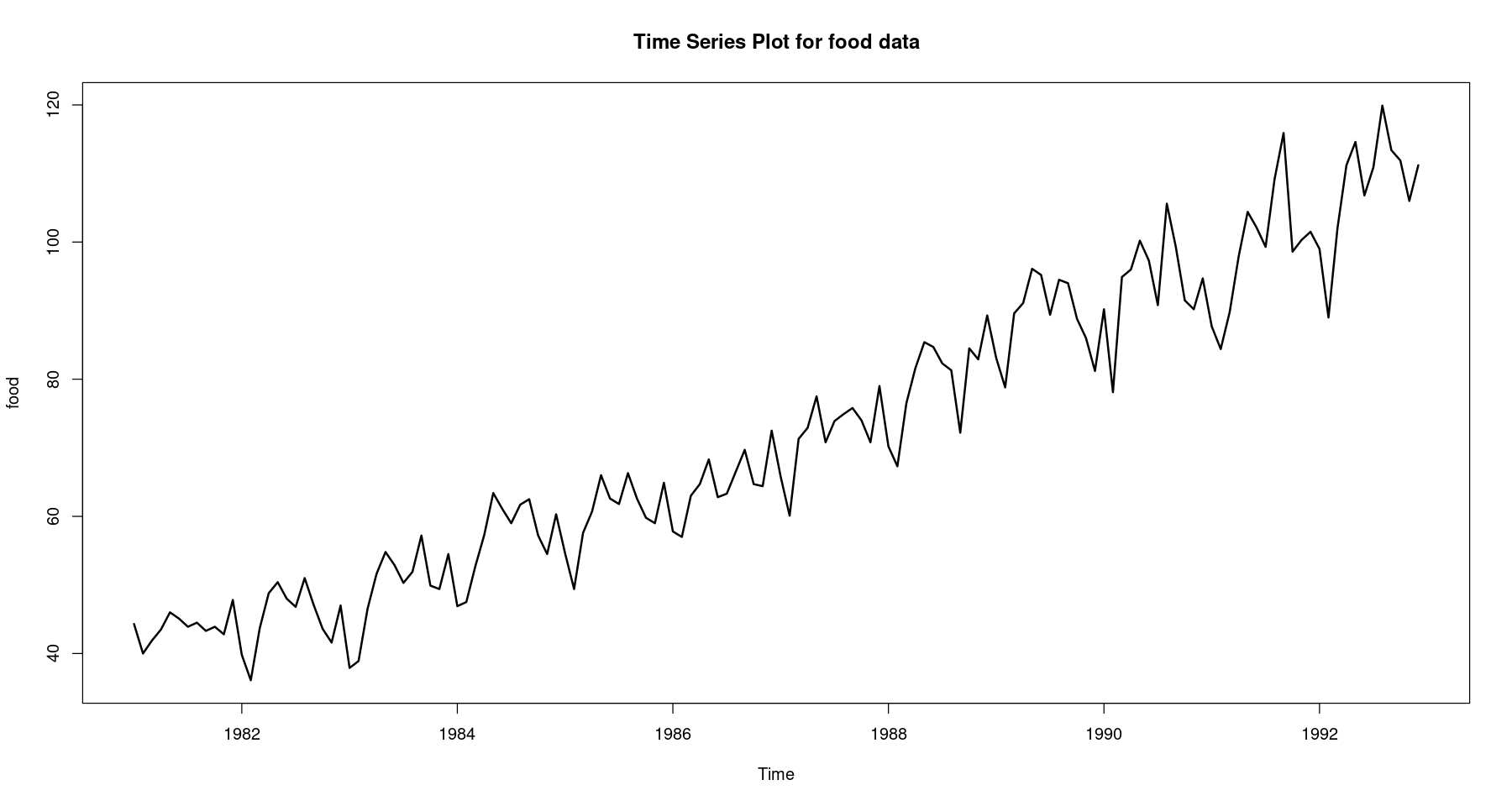
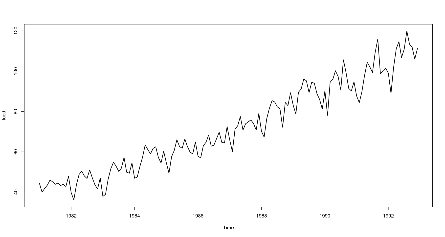
<- scan ("food.txt" )<- 1 : length (z)<- ts (z, start= c (1981 ,1 ), frequency= 12 )plot.ts (food, lwd= 2 , main = "Time Series Plot for food data" )
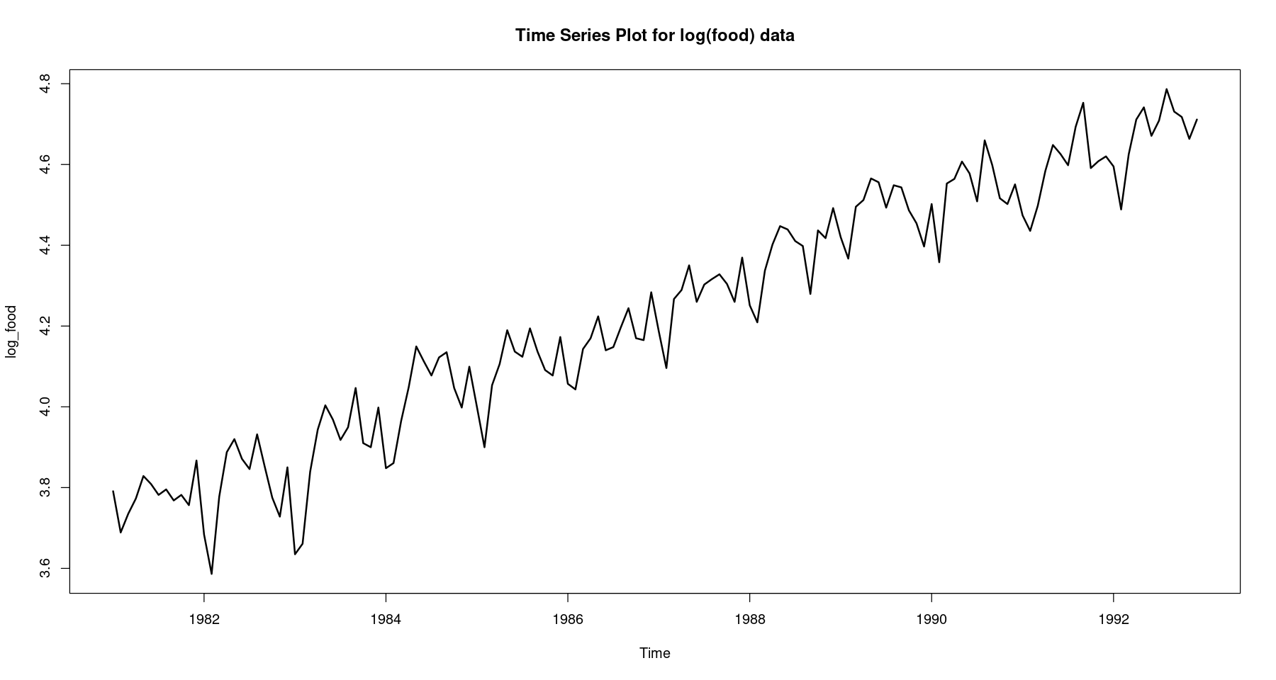
## 이분산성 제거를 위한 변수 변환 <- log (food)plot.ts (log_food, lwd= 2 , main = "Time Series Plot for log(food) data" )
진폭이 시간의 흐름에 따라 거의 일정해 진 것을 확인할 수 있음
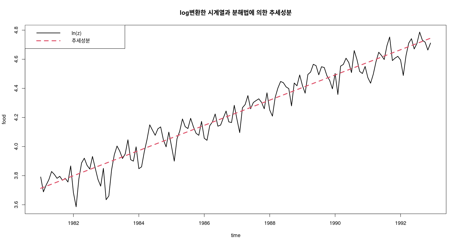
1. 추세성분 추정: \(Z_t = \beta_0 + \beta_1t + \epsilon_t\) 적합
<- lm (log_food ~ t ) summary (fit)
Call:
lm(formula = log_food ~ t)

Residuals:
      Min        1Q    Median        3Q       Max
-0.251154 -0.042190  0.009368  0.051058  0.147910

Coefficients:
            Estimate Std. Error t value Pr(>|t|)
(Intercept) 3.705715   0.012870  287.94   <2e-16 ***
t           0.007216   0.000154   46.86   <2e-16 ***
---
Signif. codes:  0 ‘***’ 0.001 ‘**’ 0.01 ‘*’ 0.05 ‘.’ 0.1 ‘ ’ 1

Residual standard error: 0.07682 on 142 degrees of freedom
Multiple R-squared:  0.9393,    Adjusted R-squared:  0.9388
F-statistic:  2195 on 1 and 142 DF,  p-value: < 2.2e-16
\(\hat{T}_t = 3.706 + 0.007t\)
<- fitted (fit)ts.plot (log_food, hat_Tt,col= 1 : 2 ,lty= 1 : 2 ,lwd= 2 : 3 ,ylab= "food" , xlab= "time" ,main= "log변환한 시계열과 분해법에 의한 추세성분" )legend ("topleft" , lty= 1 : 2 , col= 1 : 2 , lwd= 2 : 3 , c ("ln(z)" , "추세성분" ))
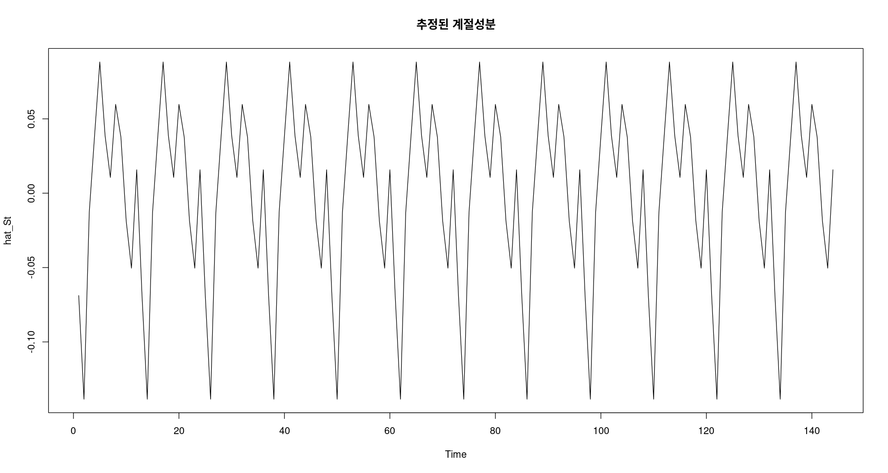
2. 계절성분 추정 \(Z_t-\hat{T}_t = \delta_1I_1 + \dots + \delta_{12} I_{12} + \epsilon_t\) : 적합
위에서 지시함수를 이용하여 모형 적합
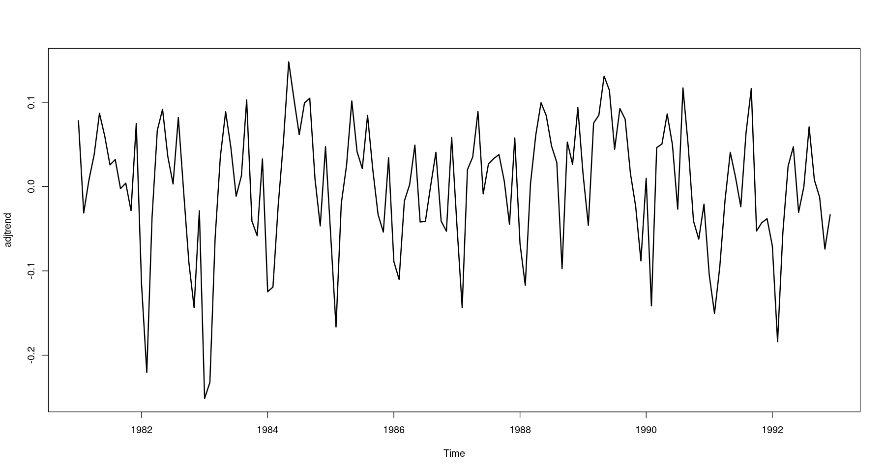
## 원시계열에서 추세성분 조정 = log_food- hat_Ttplot.ts (adjtrend, lwd= 2 )
## 지시함수를 이용한 계절성분 추정 = factor (cycle (adjtrend)) #범주형 변수로 변환 <- lm (adjtrend ~ 0 + y)summary (fit1)
Call:
lm(formula = adjtrend ~ 0 + y)

Residuals:
      Min        1Q    Median        3Q       Max
-0.182321 -0.028501  0.000597  0.025663  0.146887

Coefficients:
    Estimate Std. Error t value Pr(>|t|)
y1  -0.06883    0.01423  -4.837 3.61e-06 ***
y2  -0.13853    0.01423  -9.735  < 2e-16 ***
y3  -0.01290    0.01423  -0.907 0.366289
y4   0.03840    0.01423   2.699 0.007872 **
y5   0.08825    0.01423   6.201 6.69e-09 ***
y6   0.03871    0.01423   2.720 0.007401 **
y7   0.01061    0.01423   0.746 0.457221
y8   0.05972    0.01423   4.197 4.94e-05 ***
y9   0.03776    0.01423   2.653 0.008945 **
y10 -0.01856    0.01423  -1.304 0.194518
y11 -0.05041    0.01423  -3.542 0.000549 ***
y12  0.01577    0.01423   1.108 0.269816
---
Signif. codes:  0 ‘***’ 0.001 ‘**’ 0.01 ‘*’ 0.05 ‘.’ 0.1 ‘ ’ 1

Residual standard error: 0.0493 on 132 degrees of freedom
Multiple R-squared:  0.6172,    Adjusted R-squared:  0.5824
F-statistic: 17.73 on 12 and 132 DF,  p-value: < 2.2e-16
<- fitted (fit1)ts.plot (hat_St, main= "추정된 계절성분" )
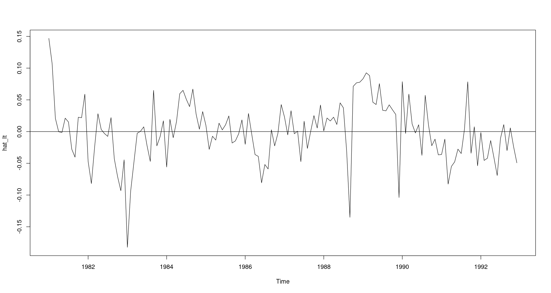
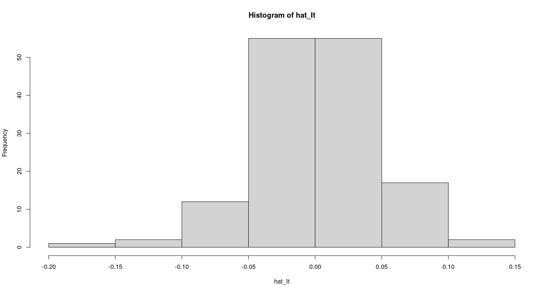
3. 불규칙 성분 \(\hat{I}_t = Z_t - \hat{T}_t - \hat{S}_t\)
<- log_food - hat_Tt - hat_Stts.plot (hat_It); abline (h= 0 )
t.test (hat_It) #H0 : mu=E(It)=0
    One Sample t-test

data:  hat_It
t = 5.9991e-16, df = 143, p-value = 1
alternative hypothesis: true mean is not equal to 0
95 percent confidence interval:
 -0.007801616  0.007801616
sample estimates:
   mean of x
2.367739e-18
귀무가설을 기각할 수 없다. 즉 평균이 0이다.
dwtest (lm (hat_It~ 1 ),alternative = 'two.sided' )
    Durbin-Watson test

data:  lm(hat_It ~ 1)
DW = 1.0803, p-value = 2.748e-08
alternative hypothesis: true autocorrelation is not 0
bptest이용해서 등분산성/이분사넛ㅇ 확인해야함.. -> 자꾸 오류나넹
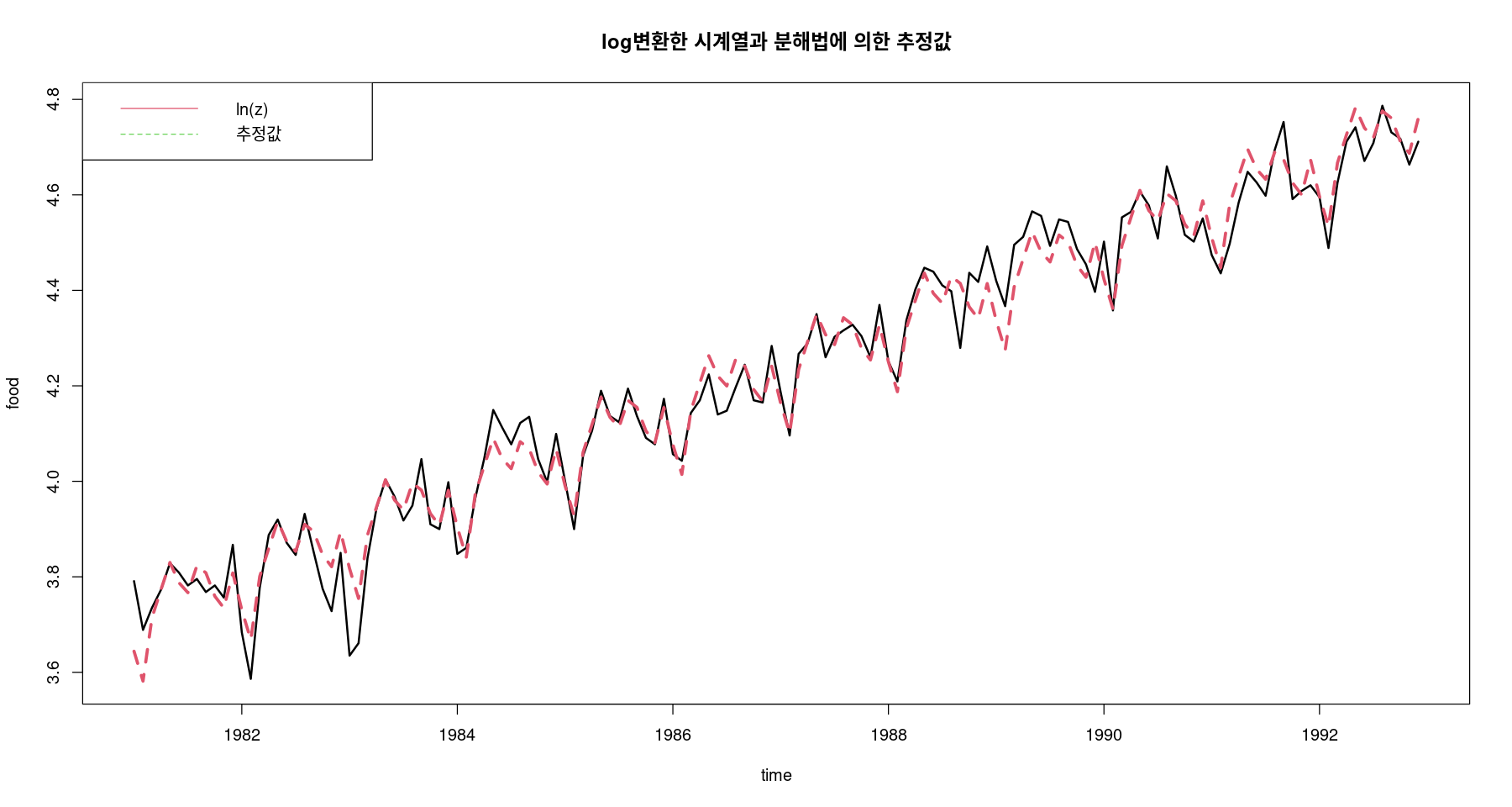
4. 추정 \(\hat{Z}_t = \hat{T}_t + \hat{S}_t\)
체계적 성분: 추세, 계절 성분
비체계적 성분: 불규칙 성분
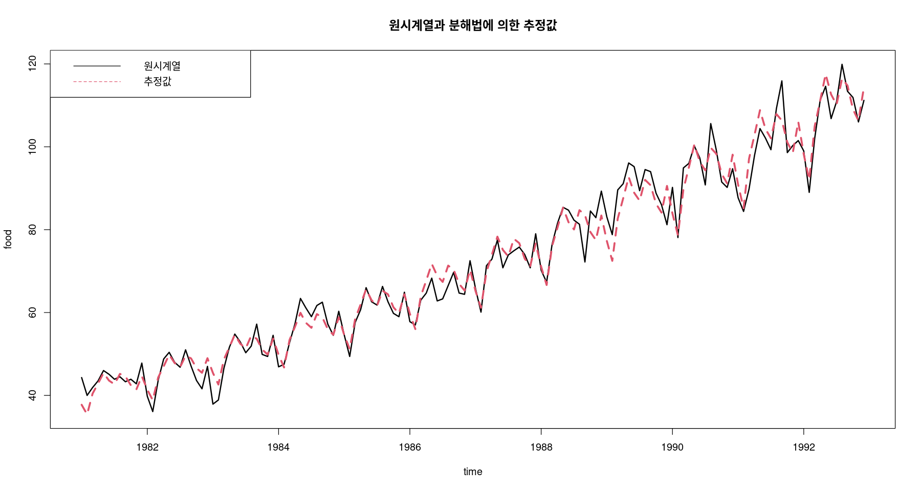
<- hat_Tt + hat_Stts.plot (log_food, pred_a, col= 1 : 2 , lty= 1 : 2 , lwd= 2 : 3 ,ylab= "food" , xlab= "time" ,main= "log변환한 시계열과 분해법에 의한 추정값" )legend ("topleft" , lty= 1 : 2 , col= 2 : 3 , c ("ln(z)" , "추정값" ))
ts.plot (food, exp (pred_a), col= 1 : 2 , lty= 1 : 2 , lwd= 2 : 3 ,ylab= "food" , xlab= "time" ,main= "시계열과 분해법에 의한 추정값" )legend ("topleft" , lty= 1 : 2 , col= 1 : 2 , c ("Z" , "추정값" ))
SSE/MSE 구할 때 로그 변환 했던 데이터 -> 오리지널 데이터로 변환해서 비교해야함!!!
= sum ((food- exp (pred_a))^ 2 )= mean ((food- exp (pred_a))^ 2 )
1636.87967934919
11.3672199954805
추세를 이용한 분해법 - 승법모형
\(Z_t = T_t \times S_t \times I_t\) , 계절주기:s
1. 추세성분 추정: \(Z_t = \beta_0 + \beta_1t + \epsilon_t\) 적합
## 추세성분 추정 <- lm (food ~ t ) summary (fit3)
Call:
lm(formula = food ~ t)

Residuals:
     Min       1Q   Median       3Q      Max
-14.0331  -3.4505  -0.1355   4.2911  15.3948

Coefficients:
            Estimate Std. Error t value Pr(>|t|)
(Intercept) 35.28614    0.95561   36.92   <2e-16 ***
t            0.50557    0.01143   44.21   <2e-16 ***
---
Signif. codes:  0 ‘***’ 0.001 ‘**’ 0.01 ‘*’ 0.05 ‘.’ 0.1 ‘ ’ 1

Residual standard error: 5.704 on 142 degrees of freedom
Multiple R-squared:  0.9323,    Adjusted R-squared:  0.9318
F-statistic:  1955 on 1 and 142 DF,  p-value: < 2.2e-16
\(\hat{T}_t = 35.286 + 0.506t\)
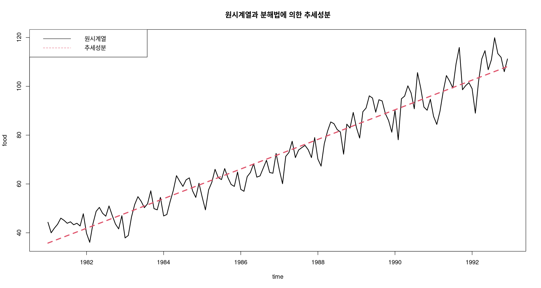
ts.plot (food, fitted (fit3) , col= 1 : 2 , lty= 1 : 2 , lwd= 2 : 3 , ylab= "food" , xlab= "time" ,main= "원시계열과 분해법에 의한 추세성분" )legend ("topleft" , lty= 1 : 2 , col= 1 : 2 , c ("원시계열" , "추세성분" ))
<- lm (food ~ t+ I (t^ 2 )) summary (fit4)
Call:
lm(formula = food ~ t + I(t^2))

Residuals:
    Min      1Q  Median      3Q     Max
-16.845  -3.535   0.566   3.523  13.391

Coefficients:
             Estimate Std. Error t value Pr(>|t|)
(Intercept) 4.011e+01  1.346e+00  29.799  < 2e-16 ***
t           3.071e-01  4.286e-02   7.166 3.96e-11 ***
I(t^2)      1.369e-03  2.863e-04   4.779 4.37e-06 ***
---
Signif. codes:  0 ‘***’ 0.001 ‘**’ 0.01 ‘*’ 0.05 ‘.’ 0.1 ‘ ’ 1

Residual standard error: 5.31 on 141 degrees of freedom
Multiple R-squared:  0.9417,    Adjusted R-squared:  0.9409
F-statistic:  1139 on 2 and 141 DF,  p-value: < 2.2e-16
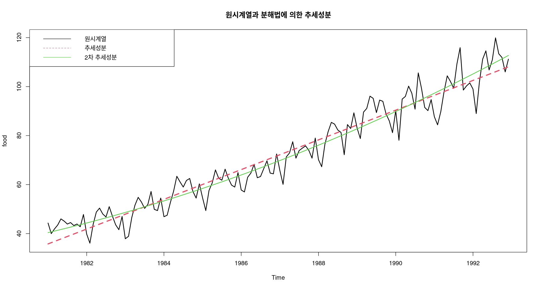
ts.plot (food, fitted (fit3), fitted (fit4), col= 1 : 3 , lty= 1 : 2 , lwd= 2 : 3 , ylab= "food" ,main= "원시계열과 분해법에 의한 추세성분" )legend ("topleft" , lty= 1 : 2 , col= 1 : 3 , c ("원시계열" , "추세성분" , "2차 추세성분" ))
2. 계절성분 추정 \(Z_t / \hat{T}_t = \delta_1I_1 + \dots + \delta_{12} I_{12} + \epsilon_t\) : 적합
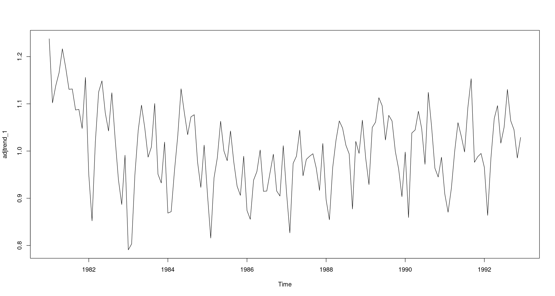
## 원시계열에서 추세성분 조정 = fitted (fit3) # fit3:1차 추세모형 = food/ trend_1plot.ts (adjtrend_1)
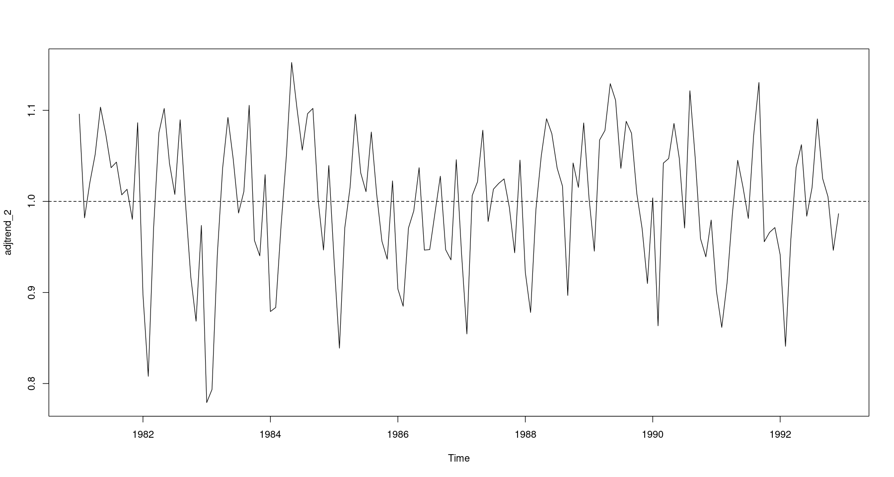
## 원시계열에서 2차 추세성분 조정 = fitted (fit4) # fit4: 2차 추세모형 = food/ trend_2plot.ts (adjtrend_2)abline (h= 1 , lty= 2 )
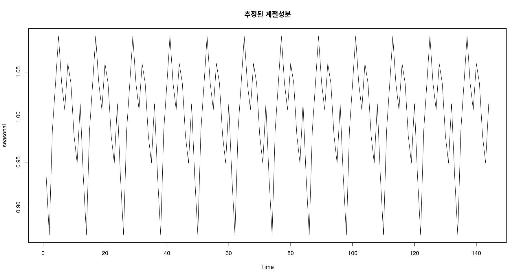
## 지시함수를 이용한 계절성분 추정 = factor (cycle (adjtrend_2)) <- lm (adjtrend_2 ~ 0 + y)summary (fit5)
Call:
lm(formula = adjtrend_2 ~ 0 + y)

Residuals:
      Min        1Q    Median        3Q       Max
-0.154659 -0.027736  0.000622  0.028345  0.162186

Coefficients:
    Estimate Std. Error t value Pr(>|t|)
y1   0.93372    0.01368   68.23   <2e-16 ***
y2   0.86951    0.01368   63.54   <2e-16 ***
y3   0.98517    0.01368   72.00   <2e-16 ***
y4   1.03650    0.01368   75.75   <2e-16 ***
y5   1.08954    0.01368   79.62   <2e-16 ***
y6   1.03763    0.01368   75.83   <2e-16 ***
y7   1.00829    0.01368   73.69   <2e-16 ***
y8   1.05940    0.01368   77.42   <2e-16 ***
y9   1.03744    0.01368   75.82   <2e-16 ***
y10  0.97966    0.01368   71.59   <2e-16 ***
y11  0.94903    0.01368   69.35   <2e-16 ***
y12  1.01466    0.01368   74.15   <2e-16 ***
---
Signif. codes:  0 ‘***’ 0.001 ‘**’ 0.01 ‘*’ 0.05 ‘.’ 0.1 ‘ ’ 1

Residual standard error: 0.0474 on 132 degrees of freedom
Multiple R-squared:  0.998, Adjusted R-squared:  0.9978
F-statistic:  5359 on 12 and 132 DF,  p-value: < 2.2e-16
\(\hat{S}_t = 0.934I_1 + 0.870I_2 + ⋯ + 1.015I_{12}\)
<- fitted (fit5)ts.plot (seasonal, main= "추정된 계절성분" )
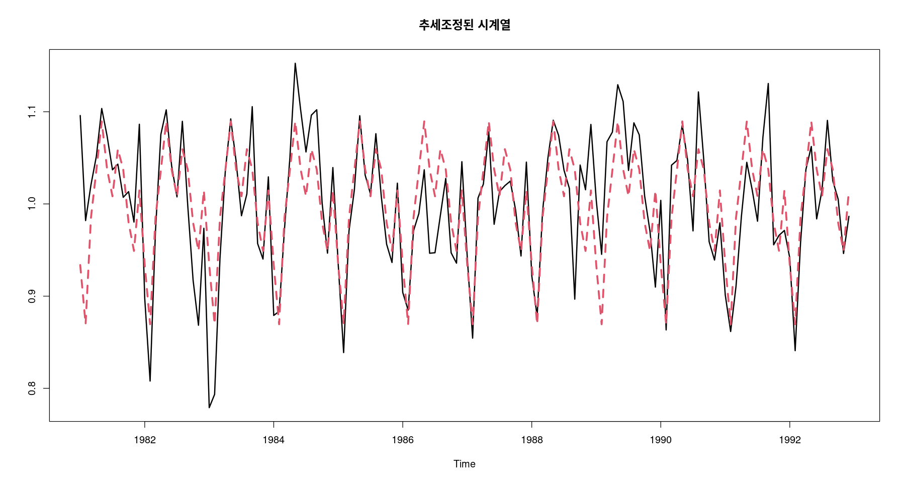
<- fitted (fit5)ts.plot (adjtrend_2, seasonal, col= 1 : 2 , lty= 1 : 2 , lwd= 2 : 3 , main= "추세조정된 시계열" )
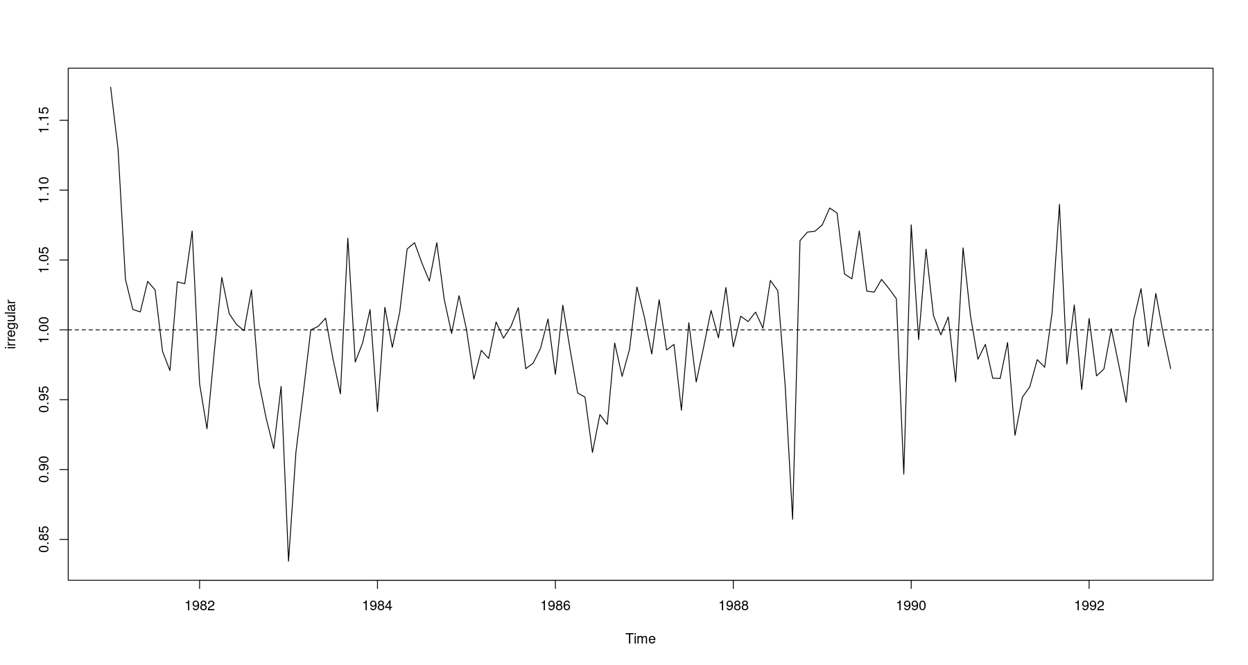
3. 불규칙 성분 \(\hat{I}_t = Z_t / ( \hat{T}_t \times \hat{S}_t)\)
<- food/ trend_2/ seasonalts.plot (irregular); abline (h= 1 , lty= 2 )
    One Sample t-test

data:  irregular
t = 0, df = 143, p-value = 1
alternative hypothesis: true mean is not equal to 1
95 percent confidence interval:
 0.9923514 1.0076486
sample estimates:
mean of x
        1
나눠준거기 떄문에.. 비슷하면 1이랑 가까워지니까 mu=1과 비교하는 것
dwtest (lm (irregular~ 1 ), alternative = 'two.sided' )
    Durbin-Watson test

data:  lm(irregular ~ 1)
DW = 1.0897, p-value = 3.799e-08
alternative hypothesis: true autocorrelation is not 0
4. 추정 \(\hat{Z}_t = \hat{T}_t \times \hat{S}_t\)
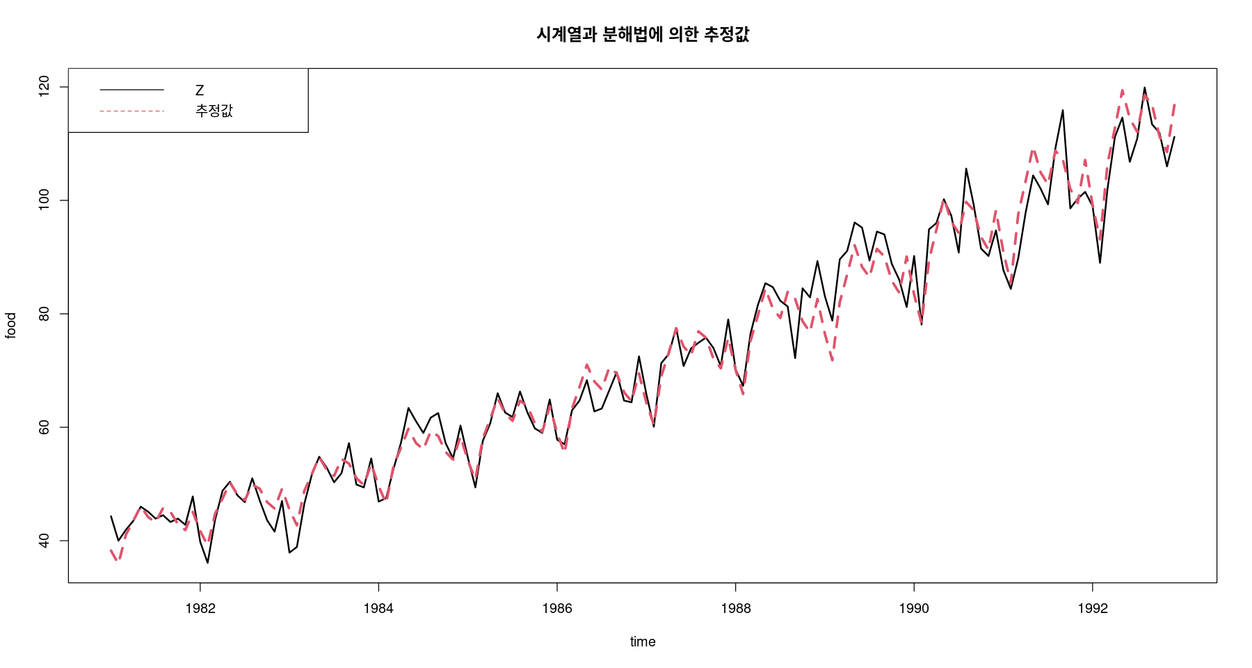
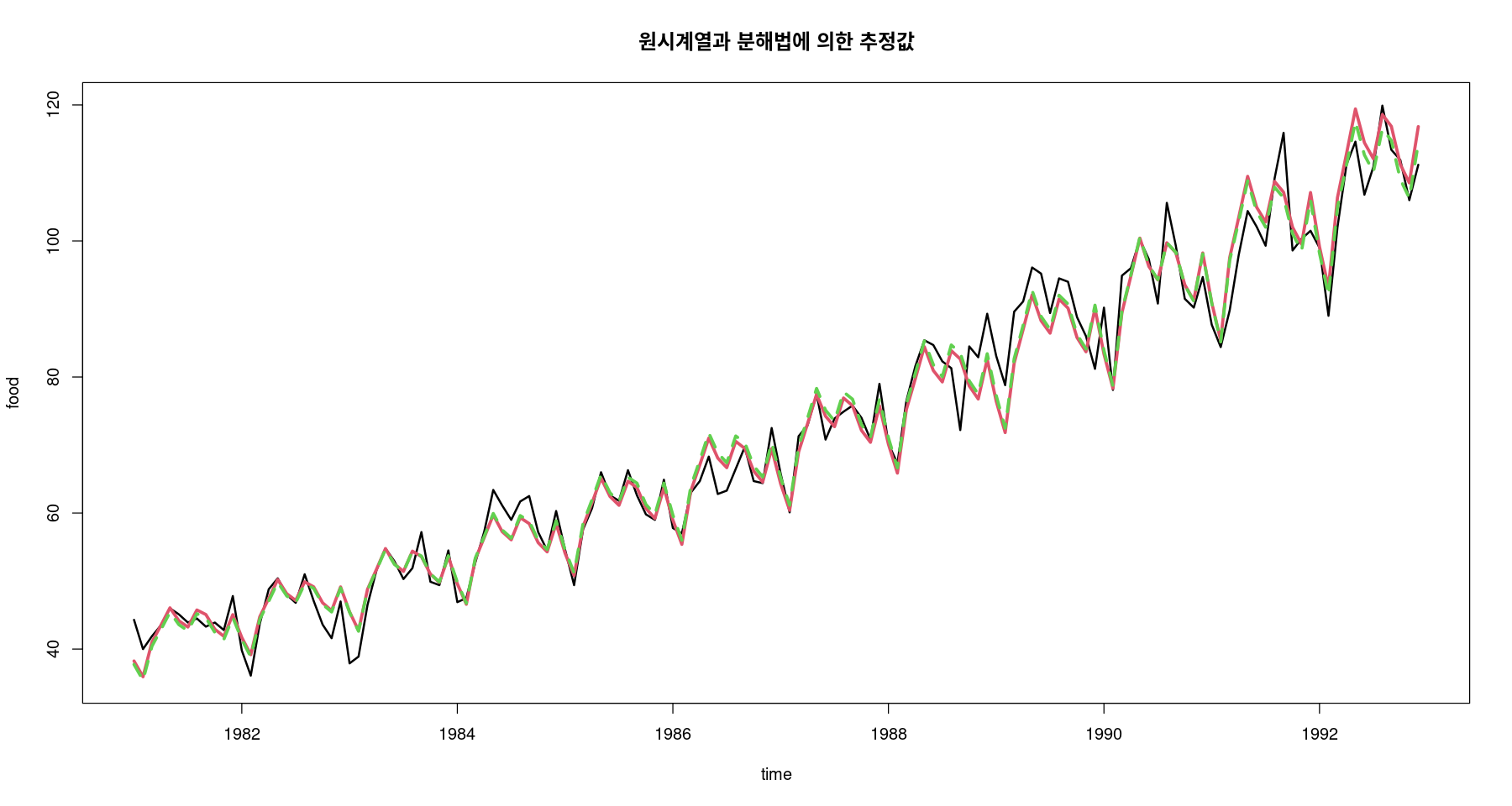
<- trend_2 * seasonalts.plot (food, pred_m, col= 1 : 2 , lty= 1 : 2 , lwd= 2 : 3 , ylab= "food" , xlab= "time" ,main= "원시계열과 분해법에 의한 추정값" )legend ("topleft" , lty= 1 : 2 , col= 1 : 2 , c ("원시계열" , "추정값" ))
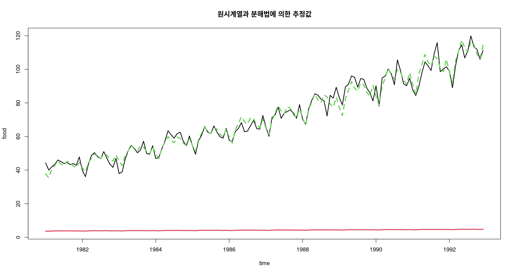
#pred_a #가법 #pred_m #승법 ts.plot (food, pred_a, pred_m, col= 1 : 3 , lty= c (1 ,1 ,2 ), lwd= c (2 ,3 ,3 ), ylab= "food" , xlab= "time" ,main= "원시계열과 분해법에 의한 추정값" )
pred_a는 원 food데이터에서 log를 취한 값이라 그런지,, 빨간색 선..
#pred_a #가법 #pred_m #승법 ts.plot (food, exp (pred_a), pred_m, col= 1 : 3 , lty= c (1 ,1 ,2 ), lwd= c (2 ,3 ,3 ), ylab= "food" , xlab= "time" ,main= "원시계열과 분해법에 의한 추정값" )
SSE/MSE비교
#가법 sum ((food- exp (pred_a))^ 2 ) ##SSE mean ((food- exp (pred_a))^ 2 ) ##MSE
1636.87967934919
11.3672199954805
#승법 sum ((food- pred_m)^ 2 ) #SSE mean ((food- pred_m)^ 2 ) #MSE
1483.03817025796
10.298876182347